install.packages('tidyverse')3 Manipulating and analyzing data
3.1 Lesson preamble
3.1.1 Learning objectives
- Load external data from a .csv file into a data frame in R using
read_csv- Describe what a
data frameis- Learn multiple ways to “index” (ie., the values from) data frames
- Understand the purpose of the dplyr package.
- Use dplyr functions to summarize the contents of data frames (e.g.,
str,head,tail,summary,dim,ncol,nrow,colnames,rownames)- Learn to use data wrangling commands
select,filter,andmutatefrom the dplyr package- Create multi-step data-manipulation processes using pipes (
%>%)to chains steps together
3.2 Set up
To do this lecture, we’ll need to be able to create and knit R Markdown documents, and analyze data using functions contained in the tidyverse package. If you haven’t done either of these tasks before, navigate to the course notes for Lecture 1 and follow the instructions there first. Then, open a new document (File > New File > R Markdown) to run commands during this lecture.
When we make Markdown documents, we want them to be shareable and reproducible, so it’s good practice to include code to install and load any packages the code requires, even if we’ve already done it ourselves. While packages only need to be installed once (they’ll still be there even if RStudio is closed and reopened again or if R is accessed outside of RStudio), someone we share our code with might have never used them before. Or, if you move from using your code on one computer to another, or one computer to the POSIT Cloud, you’ll need to re-install.
We can add code install new packages using the function install.packages(). We’ll pass eval=FALSE to knitr at the top of our code chunk to make sure that the chunk won’t be evaluated when we knit the document, since we don’t really need to install it each time, and this option can be changed by another user. You can find other possible options to pass that can be helpful for formatting your output document.
The two tidyverse packages we will be using the most frequently in this course is dplyr and ggplot2. dplyr is great for data wrangling (Lecture 3) and ggplot2 makes killer plots (Lecture 4).
To use functions in the dplyr package, type dplyr:: and then the function name.
dplyr::glimpse(cars) # `glimpse` is similar to `str`Rows: 50
Columns: 2
$ speed <dbl> 4, 4, 7, 7, 8, 9, 10, 10, 10, 11, 11, 12, 12, 12, 12, 13, 13, 13…
$ dist <dbl> 2, 10, 4, 22, 16, 10, 18, 26, 34, 17, 28, 14, 20, 24, 28, 26, 34…# cars is a built-in data setSince we will be using this package a lot, it would be a little annoying to have to type dplyr:: every time. We can bypass this step by loading the package into our current environment. Think of this is “opening” the package for your work session.
# We could also do `library(dplyr)`, but we need the rest of the
# tidyverse packages later, so we might as well import the entire collection.library(tidyverse)── Attaching core tidyverse packages ──────────────────────── tidyverse 2.0.0 ──
✔ dplyr 1.1.4 ✔ readr 2.1.6
✔ forcats 1.0.1 ✔ stringr 1.6.0
✔ ggplot2 4.0.1 ✔ tibble 3.3.0
✔ lubridate 1.9.4 ✔ tidyr 1.3.2
✔ purrr 1.2.0
── Conflicts ────────────────────────────────────────── tidyverse_conflicts() ──
✖ dplyr::filter() masks stats::filter()
✖ dplyr::lag() masks stats::lag()
ℹ Use the conflicted package (<http://conflicted.r-lib.org/>) to force all conflicts to become errorsglimpse(cars)Rows: 50
Columns: 2
$ speed <dbl> 4, 4, 7, 7, 8, 9, 10, 10, 10, 11, 11, 12, 12, 12, 12, 13, 13, 13…
$ dist <dbl> 2, 10, 4, 22, 16, 10, 18, 26, 34, 17, 28, 14, 20, 24, 28, 26, 34…This needs to be done once for every new R session, and so it is common practice to keep a list of all the packages used at the top of your script or notebook for convenience and load all of it at start up.
You might notice a lot of red text printed in the console! What are these warning signs and checks?
All the warning signs indicate are the version of R that they were built under. They can frequently be ignored unless your version of R is so old that the packages can no longer be run on R! Note that packages are frequently updated, and functions may become deprecated.
Next, the warning shows you all the packages that were successfully installed.
Finally, there are usually some conflicts reported. All this means is that there are multiple functions with the same name that may do different things. R prioritizes functions from certain packages over others. So, in this case, the filter() function from dplyr will take precedent over the filter() function from the stats package. If you want to use the latter, use double colons :: to indicate that you are calling a function from a certain package:
3.3 Dataset background
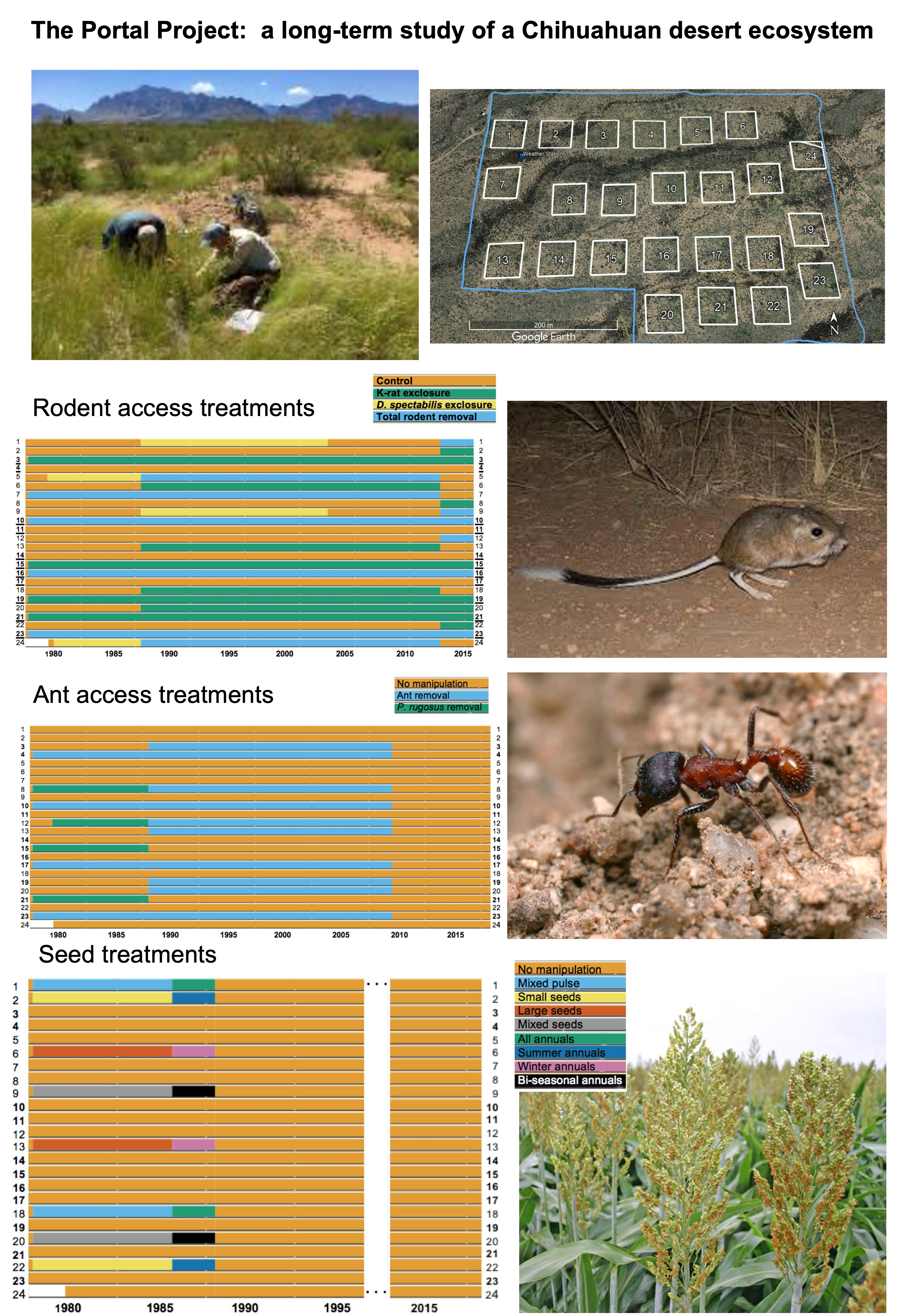
Today, we will be working with real data from a longitudinal study of the species abundance in the Chihuahuan desert ecosystem near Portal, Arizona, USA. This study includes observations of plants, ants, and rodents from 1977 - 2002, and has been used in over 100 publications.
More information is available in the abstract of this paper from 2009, in this pre-print, and on the Portal Project’s website. There are several datasets available related to this study, and we will be working with datasets that have been preprocessed by the Data Carpentry to facilitate teaching. These are made available online as The Portal Project Teaching Database, both at the Data Carpentry website, and on Figshare. Figshare is a great place to publish data, code, figures, and more openly to make them available for other researchers and to communicate findings that are not part of a longer paper.
3.3.1 Presentation of the survey data
We are studying the species and weight of animals caught in plots in our study area. The dataset is stored as a comma separated value (CSV) file. Each row holds information for a single animal, and the columns represent:
| Column | Description |
|---|---|
| record_id | unique id for the observation |
| month | month of observation |
| day | day of observation |
| year | year of observation |
| plot_id | ID of a particular plot |
| species_id | 2-letter code |
| sex | sex of animal (“M”, “F”) |
| hindfoot_length | length of the hindfoot in mm |
| weight | weight of the animal in grams |
| genus | genus of animal |
| species | species of animal |
| taxa | e.g. rodent, reptile, bird, rabbit |
| plot_type | type of plot |
To read the data into R, we are going to use a function called read_csv. This function is contained in an R-package called readr. R-packages are a bit like browser extensions; they are not essential, but can provide nifty functionality. We will go through R-packages in general and which ones are good for data analyses. One useful option that read_csv includes, is the ability to read a CSV file directly from a URL, without downloading it in a separate step:
library(readr)surveys <- readr::read_csv('https://ndownloader.figshare.com/files/2292169')However, it is often a good idea to download the data first, so you have a copy stored locally on your computer in case you want to do some offline analyses, or the online version of the file changes or the file is taken down. You can either download the data manually or from within R:
download.file("https://ndownloader.figshare.com/files/2292169",
              "data/portal_data.csv") # Saves to current directory with this name
The data is read in by specifying its local path.
surveys <- readr::read_csv('data/portal_data.csv')Rows: 34786 Columns: 13
── Column specification ────────────────────────────────────────────────────────
Delimiter: ","
chr (6): species_id, sex, genus, species, taxa, plot_type
dbl (7): record_id, month, day, year, plot_id, hindfoot_length, weight
ℹ Use `spec()` to retrieve the full column specification for this data.
ℹ Specify the column types or set `show_col_types = FALSE` to quiet this message.This statement produces some output regarding which data type it found in each column. If we want to check this in more detail, we can print the variable’s value: surveys.
surveys# A tibble: 34,786 × 13
record_id month day year plot_id species_id sex hindfoot_length weight
<dbl> <dbl> <dbl> <dbl> <dbl> <chr> <chr> <dbl> <dbl>
1 1 7 16 1977 2 NL M 32 NA
2 72 8 19 1977 2 NL M 31 NA
3 224 9 13 1977 2 NL <NA> NA NA
4 266 10 16 1977 2 NL <NA> NA NA
5 349 11 12 1977 2 NL <NA> NA NA
6 363 11 12 1977 2 NL <NA> NA NA
7 435 12 10 1977 2 NL <NA> NA NA
8 506 1 8 1978 2 NL <NA> NA NA
9 588 2 18 1978 2 NL M NA 218
10 661 3 11 1978 2 NL <NA> NA NA
# ℹ 34,776 more rows
# ℹ 4 more variables: genus <chr>, species <chr>, taxa <chr>, plot_type <chr>This displays a nice tabular view of the data, which also includes pagination when there are many rows and we can click the arrow to view all the columns. Technically, this object is actually a tibble rather than a data frame, as indicated in the output. The reason for this is that read_csv automatically converts the data into to a tibble when loading it. Since a tibble is just a data frame with some convenient extra functionality, we will use these words interchangeably from now on.
If we just want to glance at how the data frame looks, it is sufficient to display only the top (the first 6 lines) using the function head():
head(surveys)# A tibble: 6 × 13
record_id month day year plot_id species_id sex hindfoot_length weight
<dbl> <dbl> <dbl> <dbl> <dbl> <chr> <chr> <dbl> <dbl>
1 1 7 16 1977 2 NL M 32 NA
2 72 8 19 1977 2 NL M 31 NA
3 224 9 13 1977 2 NL <NA> NA NA
4 266 10 16 1977 2 NL <NA> NA NA
5 349 11 12 1977 2 NL <NA> NA NA
6 363 11 12 1977 2 NL <NA> NA NA
# ℹ 4 more variables: genus <chr>, species <chr>, taxa <chr>, plot_type <chr>3.4 What are data frames?
Data frames are the de facto data structure for most tabular data, and what we use for statistics and plotting. A data frame can be created by hand, but most commonly they are generated by the function read_csv(); in other words, when importing spreadsheets from your hard drive (or the web).
A data frame is a representation of data in the format of a table where the columns are vectors that all have the same length. Because the columns are vectors, they all contain the same type of data as we discussed in last class (e.g., characters, integers, factors). We can see this when inspecting the structure of a data frame with the function str():
str(surveys)spc_tbl_ [34,786 × 13] (S3: spec_tbl_df/tbl_df/tbl/data.frame)
$ record_id : num [1:34786] 1 72 224 266 349 363 435 506 588 661 ...
$ month : num [1:34786] 7 8 9 10 11 11 12 1 2 3 ...
$ day : num [1:34786] 16 19 13 16 12 12 10 8 18 11 ...
$ year : num [1:34786] 1977 1977 1977 1977 1977 ...
$ plot_id : num [1:34786] 2 2 2 2 2 2 2 2 2 2 ...
$ species_id : chr [1:34786] "NL" "NL" "NL" "NL" ...
$ sex : chr [1:34786] "M" "M" NA NA ...
$ hindfoot_length: num [1:34786] 32 31 NA NA NA NA NA NA NA NA ...
$ weight : num [1:34786] NA NA NA NA NA NA NA NA 218 NA ...
$ genus : chr [1:34786] "Neotoma" "Neotoma" "Neotoma" "Neotoma" ...
$ species : chr [1:34786] "albigula" "albigula" "albigula" "albigula" ...
$ taxa : chr [1:34786] "Rodent" "Rodent" "Rodent" "Rodent" ...
$ plot_type : chr [1:34786] "Control" "Control" "Control" "Control" ...
- attr(*, "spec")=
.. cols(
.. record_id = col_double(),
.. month = col_double(),
.. day = col_double(),
.. year = col_double(),
.. plot_id = col_double(),
.. species_id = col_character(),
.. sex = col_character(),
.. hindfoot_length = col_double(),
.. weight = col_double(),
.. genus = col_character(),
.. species = col_character(),
.. taxa = col_character(),
.. plot_type = col_character()
.. )
- attr(*, "problems")=<externalptr> Integer refers to a whole number, such as 1, 2, 3, 4, etc. Numbers with decimals, 1.0, 2.4, 3.333, are referred to as floats. Factors are used to represent categorical data. Factors can be ordered or unordered, and understanding them is necessary for statistical analysis and for plotting. Factors are stored as integers, and have labels (text) associated with these unique integers. While factors look (and often behave) like character vectors, they are actually integers under the hood, and you need to be careful when treating them like strings.
3.4.1 Inspecting data.frame objects
We already saw how the functions head() and str() can be useful to check the content and the structure of a data frame. Here is a non-exhaustive list of functions to get a sense of the content/structure of the data. Let’s try them out!
- Size:
dim(surveys)- returns a vector with the number of rows in the first element and the number of columns as the second element (the dimensions of the object)nrow(surveys)- returns the number of rowsncol(surveys)- returns the number of columns
- Content:
head(surveys)- shows the first 6 rowstail(surveys)- shows the last 6 rows
- Names:
names(surveys)- returns the column names (synonym ofcolnames()fordata.frameobjects)rownames(surveys)- returns the row names
- Summary:
str(surveys)- structure of the object and information about the class, length, and content of each columnsummary(surveys)- summary statistics for each column
Note: most of these functions are “generic”, they can be used on other types of objects besides data.frame.
3.4.1.1 Challenge
Based on the output of str(surveys), can you answer the following questions?
- What is the class of the object
surveys? - How many rows and how many columns are in this object?
- What range of years are included in this dataset?
- What is the mean hindfoot length of all observed animals?
3.4.2 Indexing and subsetting data frames
Our survey data frame has rows and columns (it has 2 dimensions). If we want to extract some specific data from it, we need to specify the “coordinates” we want from it. Row numbers come first, followed by column numbers. When indexing, base R data frames return a different format depending on how we index the data (i.e. either a vector or a data frame), but with enhanced data frames, tibbles, the returned object is almost always a data frame.
surveys[1, 1] # first element in the first column of the data frame# A tibble: 1 × 1
record_id
<dbl>
1 1surveys[1, 6] # first element in the 6th column# A tibble: 1 × 1
species_id
<chr>
1 NL surveys[, 1] # first column in the data frame# A tibble: 34,786 × 1
record_id
<dbl>
1 1
2 72
3 224
4 266
5 349
6 363
7 435
8 506
9 588
10 661
# ℹ 34,776 more rowssurveys[1] # first column in the data frame# A tibble: 34,786 × 1
record_id
<dbl>
1 1
2 72
3 224
4 266
5 349
6 363
7 435
8 506
9 588
10 661
# ℹ 34,776 more rowssurveys[1:3, 7] # first three elements in the 7th column# A tibble: 3 × 1
sex
<chr>
1 M
2 M
3 <NA> surveys[3, ] # the 3rd element for all columns# A tibble: 1 × 13
record_id month day year plot_id species_id sex hindfoot_length weight
<dbl> <dbl> <dbl> <dbl> <dbl> <chr> <chr> <dbl> <dbl>
1 224 9 13 1977 2 NL <NA> NA NA
# ℹ 4 more variables: genus <chr>, species <chr>, taxa <chr>, plot_type <chr>surveys[1:6, ] # equivalent to head(surveys)# A tibble: 6 × 13
record_id month day year plot_id species_id sex hindfoot_length weight
<dbl> <dbl> <dbl> <dbl> <dbl> <chr> <chr> <dbl> <dbl>
1 1 7 16 1977 2 NL M 32 NA
2 72 8 19 1977 2 NL M 31 NA
3 224 9 13 1977 2 NL <NA> NA NA
4 266 10 16 1977 2 NL <NA> NA NA
5 349 11 12 1977 2 NL <NA> NA NA
6 363 11 12 1977 2 NL <NA> NA NA
# ℹ 4 more variables: genus <chr>, species <chr>, taxa <chr>, plot_type <chr>: is a special operator that creates numeric vectors of integers in increasing or decreasing order; test 1:10 and 10:1 for instance. This works similarly to seq, which we looked at earlier in class:
0:10 [1] 0 1 2 3 4 5 6 7 8 9 10seq(0, 10) [1] 0 1 2 3 4 5 6 7 8 9 10# We can test if all elements are the same
0:10 == seq(0,10) [1] TRUE TRUE TRUE TRUE TRUE TRUE TRUE TRUE TRUE TRUE TRUEall(0:10 == seq(0,10))[1] TRUEYou can also exclude certain parts of a data frame using the “-” sign:
surveys[,-1] # All columns, except the first# A tibble: 34,786 × 12
month day year plot_id species_id sex hindfoot_length weight genus
<dbl> <dbl> <dbl> <dbl> <chr> <chr> <dbl> <dbl> <chr>
1 7 16 1977 2 NL M 32 NA Neotoma
2 8 19 1977 2 NL M 31 NA Neotoma
3 9 13 1977 2 NL <NA> NA NA Neotoma
4 10 16 1977 2 NL <NA> NA NA Neotoma
5 11 12 1977 2 NL <NA> NA NA Neotoma
6 11 12 1977 2 NL <NA> NA NA Neotoma
7 12 10 1977 2 NL <NA> NA NA Neotoma
8 1 8 1978 2 NL <NA> NA NA Neotoma
9 2 18 1978 2 NL M NA 218 Neotoma
10 3 11 1978 2 NL <NA> NA NA Neotoma
# ℹ 34,776 more rows
# ℹ 3 more variables: species <chr>, taxa <chr>, plot_type <chr>surveys[-c(7:34786),] # Equivalent to head(surveys)# A tibble: 6 × 13
record_id month day year plot_id species_id sex hindfoot_length weight
<dbl> <dbl> <dbl> <dbl> <dbl> <chr> <chr> <dbl> <dbl>
1 1 7 16 1977 2 NL M 32 NA
2 72 8 19 1977 2 NL M 31 NA
3 224 9 13 1977 2 NL <NA> NA NA
4 266 10 16 1977 2 NL <NA> NA NA
5 349 11 12 1977 2 NL <NA> NA NA
6 363 11 12 1977 2 NL <NA> NA NA
# ℹ 4 more variables: genus <chr>, species <chr>, taxa <chr>, plot_type <chr>As well as using numeric values to subset a data.frame (or matrix), columns can be called by name, using one of the four following notations:
surveys["species_id"] # Result is a data.frame# A tibble: 34,786 × 1
species_id
<chr>
1 NL
2 NL
3 NL
4 NL
5 NL
6 NL
7 NL
8 NL
9 NL
10 NL
# ℹ 34,776 more rowssurveys[, "species_id"] # Result is a data.frame# A tibble: 34,786 × 1
species_id
<chr>
1 NL
2 NL
3 NL
4 NL
5 NL
6 NL
7 NL
8 NL
9 NL
10 NL
# ℹ 34,776 more rowsFor our purposes, these notations are equivalent. RStudio knows about the columns in your data frame, so you can take advantage of the autocompletion feature to get the full and correct column name.
Another syntax that is often used to specify column names is $. In this case, the returned object is actually a vector. We will not go into detail about this, but since it is such common usage, it is good to be aware of this.
# We use `head()` since the output from vectors are not automatically cut off
# and we don't want to clutter the screen with all the `species_id` values
head(surveys$species_id)          # Result is a vector
[1] "NL" "NL" "NL" "NL" "NL" "NL"3.4.2.1 Challenge
Create a
data.frame(surveys_200) containing only the observations from row 200 of thesurveysdataset.Notice how
nrow()gave you the number of rows in adata.frame?- Use that number to pull out just that last row in the data frame.
- Compare that with what you see as the last row using
tail()to make sure it’s meeting expectations. - Pull out that last row using
nrow()instead of the row number. - Create a new data frame object (
surveys_last) from that last row.
Use
nrow()to extract the row that is in the middle of the data frame. Store the content of this row in an object namedsurveys_middle.Combine
nrow()with the-notation above to reproduce the behavior ofhead(surveys)keeping just the first through 6th rows of the surveys dataset.
3.5 Data wrangling with dplyr
Wrangling here is used in the sense of maneuvering, managing, controlling, and turning your data upside down and inside out to look at it from different angles in order to understand it. The package dplyr provides easy tools for the most common data manipulation tasks. It is built to work directly with data frames, with many common tasks optimized by being written in a compiled language (C++), this means that many operations run much faster than similar tools in R. An additional feature is the ability to work directly with data stored in an external database, such as SQL-databases. The ability to work with databases is great because you are able to work with much bigger datasets (100s of GB) than your computer could normally handle. We will not talk in detail about this in class, but there are great resources online to learn more (e.g. this lecture from Data Carpentry).
3.5.1 Selecting columns and filtering rows
We’re going to learn some of the most common dplyr functions: select(), filter(), mutate(), group_by(), and summarise(). To select columns of a data frame, use select(). The first argument to this function is the data frame (surveys), and the subsequent arguments are the columns to keep. Note that we don’t need quotation marks around the column names here like with did with base R. You do still need quotation marks around strings, though!
# A tibble: 34,786 × 4
   plot_id species_id weight  year
     <dbl> <chr>       <dbl> <dbl>
 1       2 NL             NA  1977
 2       2 NL             NA  1977
 3       2 NL             NA  1977
 4       2 NL             NA  1977
 5       2 NL             NA  1977
 6       2 NL             NA  1977
 7       2 NL             NA  1977
 8       2 NL             NA  1978
 9       2 NL            218  1978
10       2 NL             NA  1978
# ℹ 34,776 more rows
To choose rows based on a specific criteria, use filter():
# A tibble: 1,180 × 13
   record_id month   day  year plot_id species_id sex   hindfoot_length weight
       <dbl> <dbl> <dbl> <dbl>   <dbl> <chr>      <chr>           <dbl>  <dbl>
 1     22314     6     7  1995       2 NL         M                  34     NA
 2     22728     9    23  1995       2 NL         F                  32    165
 3     22899    10    28  1995       2 NL         F                  32    171
 4     23032    12     2  1995       2 NL         F                  33     NA
 5     22003     1    11  1995       2 DM         M                  37     41
 6     22042     2     4  1995       2 DM         F                  36     45
 7     22044     2     4  1995       2 DM         M                  37     46
 8     22105     3     4  1995       2 DM         F                  37     49
 9     22109     3     4  1995       2 DM         M                  37     46
10     22168     4     1  1995       2 DM         M                  36     48
# ℹ 1,170 more rows
# ℹ 4 more variables: genus <chr>, species <chr>, taxa <chr>, plot_type <chr>
3.5.1.1 An aside on conditionals
Note that to check for equality, R requires two equal signs (==). This is to prevent confusion with object assignment, since otherwise year = 1995 might be interpreted as ‘set the year parameter to 1995’, which is not what filter does!
Basic conditionals in R are broadly similar to how they’re already expressed mathematically:
2 < 3[1] TRUE5 > 9[1] FALSEHowever, there are a few idiosyncrasies to be mindful of for other conditionals:
2 != 3 # not equal[1] TRUE2 <= 3 # less than or equal to[1] TRUE5 >= 9 # greater than or equal to[1] FALSEFinally, the %in% operator is used to check for membership:
2 %in% c(2, 3, 4) # check whether 2 in c(2, 3, 4)[1] TRUEAll of the above conditionals are compatible with filter, with the key difference being that filter expects column names as part of conditional statements instead of individual numbers.
3.5.2 Chaining functions together using pipes
But what if you wanted to select and filter at the same time? There are three ways to do this: use intermediate steps, nested functions, or pipes. With intermediate steps, you essentially create a temporary data frame and use that as input to the next function. This can clutter up your workspace with lots of objects:
# A tibble: 1,180 × 4
   plot_id species_id weight  year
     <dbl> <chr>       <dbl> <dbl>
 1       2 NL             NA  1995
 2       2 NL            165  1995
 3       2 NL            171  1995
 4       2 NL             NA  1995
 5       2 DM             41  1995
 6       2 DM             45  1995
 7       2 DM             46  1995
 8       2 DM             49  1995
 9       2 DM             46  1995
10       2 DM             48  1995
# ℹ 1,170 more rows
You can also nest functions (i.e. one function inside of another). This is handy, but can be difficult to read if too many functions are nested as things are evaluated from the inside out. Readability can be mildly improved by enabling “rainbow parentheses” (open settings > Code > Display and check rainbow parentheses), but it’s still basically impossible to document and effectively convey your work with this method.
filter(select(surveys, plot_id, species_id, weight, year), year == 1995)# A tibble: 1,180 × 4
plot_id species_id weight year
<dbl> <chr> <dbl> <dbl>
1 2 NL NA 1995
2 2 NL 165 1995
3 2 NL 171 1995
4 2 NL NA 1995
5 2 DM 41 1995
6 2 DM 45 1995
7 2 DM 46 1995
8 2 DM 49 1995
9 2 DM 46 1995
10 2 DM 48 1995
# ℹ 1,170 more rowsThe last option, pipes, are a fairly recent addition to R. Pipes let you take the output of one function and send it directly to the next, which is useful when you need to do many things to the same dataset. Pipes in R look like %>% and are made available via the magrittr package that also is included in the tidyverse. If you use RStudio, you can type the pipe with Ctrl/Cmd + Shift + M.
surveys %>%
    select(., plot_id, species_id, weight, year) %>%
    filter(., year == 1995)
# A tibble: 1,180 × 4
plot_id species_id weight year
<dbl> <chr> <dbl> <dbl>
1 2 NL NA 1995
2 2 NL 165 1995
3 2 NL 171 1995
4 2 NL NA 1995
5 2 DM 41 1995
6 2 DM 45 1995
7 2 DM 46 1995
8 2 DM 49 1995
9 2 DM 46 1995
10 2 DM 48 1995
# ℹ 1,170 more rowsThe . refers to the object that is passed from the previous line. In this example, the data frame surveys is passed to the . in the select() statement. Then, the modified data frame which is the result of the select() operation, is passed to the . in the filter() statement. Put more simply: whatever was the result from the line above the current line, will be used in the current line.
Since it gets a bit tedious to write out all the dots, dplyr allows for them to be omitted. By default, the pipe will pass its input to the first argument of the right hand side function; in dplyr, the first argument is always a data frame. The chunk below gives the same output as the one above:
surveys %>%
    select(plot_id, species_id, weight, year) %>%
    filter(year == 1995)
# A tibble: 1,180 × 4
plot_id species_id weight year
<dbl> <chr> <dbl> <dbl>
1 2 NL NA 1995
2 2 NL 165 1995
3 2 NL 171 1995
4 2 NL NA 1995
5 2 DM 41 1995
6 2 DM 45 1995
7 2 DM 46 1995
8 2 DM 49 1995
9 2 DM 46 1995
10 2 DM 48 1995
# ℹ 1,170 more rowsAnother example:
surveys %>%
  filter(weight < 5) %>%
  select(species_id, sex, weight)
# A tibble: 17 × 3
species_id sex weight
<chr> <chr> <dbl>
1 PF F 4
2 PF F 4
3 PF M 4
4 RM F 4
5 RM M 4
6 PF <NA> 4
7 PP M 4
8 RM M 4
9 RM M 4
10 RM M 4
11 PF M 4
12 PF F 4
13 RM M 4
14 RM M 4
15 RM F 4
16 RM M 4
17 RM M 4In the above code, we use the pipe to send the surveys dataset first through filter() to keep rows where weight is less than 5, then through select() to keep only the species_id, sex, and weight columns. Since %>% takes the object on its left and passes it as the first argument to the function on its right, we don’t need to explicitly include it as an argument to the filter() and select() functions anymore.
If this runs off your screen and you just want to see the first few rows, you can use a pipe to view the head() of the data. (Pipes work with non-dplyr functions, too, as long as either the dplyr or magrittr package is loaded).
surveys %>%
  filter(weight < 5) %>%
  select(species_id, sex, weight) %>%
  head()
# A tibble: 6 × 3
species_id sex weight
<chr> <chr> <dbl>
1 PF F 4
2 PF F 4
3 PF M 4
4 RM F 4
5 RM M 4
6 PF <NA> 4If we wanted to create a new object with this smaller version of the data, we could do so by assigning it a new name:
surveys_sml <- surveys %>%
  filter(weight < 5) %>%
  select(species_id, sex, weight)

surveys_sml
# A tibble: 17 × 3
species_id sex weight
<chr> <chr> <dbl>
1 PF F 4
2 PF F 4
3 PF M 4
4 RM F 4
5 RM M 4
6 PF <NA> 4
7 PP M 4
8 RM M 4
9 RM M 4
10 RM M 4
11 PF M 4
12 PF F 4
13 RM M 4
14 RM M 4
15 RM F 4
16 RM M 4
17 RM M 4Note that the final data frame is the leftmost part of this expression.
A single expression can also be used to filter for several criteria, either matching all criteria (&) or any criteria (|):
surveys %>%
    filter(taxa == 'Rodent' & sex == 'F') %>%
    select(sex, taxa)
# A tibble: 15,690 × 2
sex taxa
<chr> <chr>
1 F Rodent
2 F Rodent
3 F Rodent
4 F Rodent
5 F Rodent
6 F Rodent
7 F Rodent
8 F Rodent
9 F Rodent
10 F Rodent
# ℹ 15,680 more rowssurveys %>%
filter(species == 'clarki' | species == 'leucophrys') %>%
select(species, taxa)# A tibble: 3 × 2
species taxa
<chr> <chr>
1 leucophrys Bird
2 clarki Reptile
3 leucophrys Bird 3.5.2.1 Challenge
Using pipes, subset the survey data to include individuals collected before 1995 and retain only the columns year, sex, and weight.
3.5.3 Creating new columns with mutate
Frequently, you’ll want to create new columns based on the values in existing columns. For instance, you might want to do unit conversions, or find the ratio of values in two columns. For this we’ll use mutate().
To create a new column of weight in kg:
surveys %>%
    mutate(weight_kg = weight / 1000)
# A tibble: 34,786 × 14
record_id month day year plot_id species_id sex hindfoot_length weight
<dbl> <dbl> <dbl> <dbl> <dbl> <chr> <chr> <dbl> <dbl>
1 1 7 16 1977 2 NL M 32 NA
2 72 8 19 1977 2 NL M 31 NA
3 224 9 13 1977 2 NL <NA> NA NA
4 266 10 16 1977 2 NL <NA> NA NA
5 349 11 12 1977 2 NL <NA> NA NA
6 363 11 12 1977 2 NL <NA> NA NA
7 435 12 10 1977 2 NL <NA> NA NA
8 506 1 8 1978 2 NL <NA> NA NA
9 588 2 18 1978 2 NL M NA 218
10 661 3 11 1978 2 NL <NA> NA NA
# ℹ 34,776 more rows
# ℹ 5 more variables: genus <chr>, species <chr>, taxa <chr>, plot_type <chr>,
# weight_kg <dbl>You can also create a second new column based on the first new column within the same call of mutate():
surveys %>%
    mutate(weight_kg = weight / 1000,
           weight_kg2 = weight_kg * 2)
# A tibble: 34,786 × 15
record_id month day year plot_id species_id sex hindfoot_length weight
<dbl> <dbl> <dbl> <dbl> <dbl> <chr> <chr> <dbl> <dbl>
1 1 7 16 1977 2 NL M 32 NA
2 72 8 19 1977 2 NL M 31 NA
3 224 9 13 1977 2 NL <NA> NA NA
4 266 10 16 1977 2 NL <NA> NA NA
5 349 11 12 1977 2 NL <NA> NA NA
6 363 11 12 1977 2 NL <NA> NA NA
7 435 12 10 1977 2 NL <NA> NA NA
8 506 1 8 1978 2 NL <NA> NA NA
9 588 2 18 1978 2 NL M NA 218
10 661 3 11 1978 2 NL <NA> NA NA
# ℹ 34,776 more rows
# ℹ 6 more variables: genus <chr>, species <chr>, taxa <chr>, plot_type <chr>,
# weight_kg <dbl>, weight_kg2 <dbl>The first few rows of the output are full of NAs, so if we wanted to remove those we could insert a filter() in the chain:
surveys %>%
    filter(!is.na(weight)) %>%
    mutate(weight_kg = weight / 1000)
# A tibble: 32,283 × 14
record_id month day year plot_id species_id sex hindfoot_length weight
<dbl> <dbl> <dbl> <dbl> <dbl> <chr> <chr> <dbl> <dbl>
1 588 2 18 1978 2 NL M NA 218
2 845 5 6 1978 2 NL M 32 204
3 990 6 9 1978 2 NL M NA 200
4 1164 8 5 1978 2 NL M 34 199
5 1261 9 4 1978 2 NL M 32 197
6 1453 11 5 1978 2 NL M NA 218
7 1756 4 29 1979 2 NL M 33 166
8 1818 5 30 1979 2 NL M 32 184
9 1882 7 4 1979 2 NL M 32 206
10 2133 10 25 1979 2 NL F 33 274
# ℹ 32,273 more rows
# ℹ 5 more variables: genus <chr>, species <chr>, taxa <chr>, plot_type <chr>,
# weight_kg <dbl>is.na() is a function that determines whether something is an NA. The ! symbol negates the result, so we’re asking for everything that is not an NA.
3.5.3.1 Challenge
Create a new data frame from the surveys data that meets the following criteria: contains only the species_id column and a new column called hindfoot_half containing values that are half the hindfoot_length values. In this hindfoot_half column, there are no NAs and all values are less than 30.
Hint: think about how the commands should be ordered to produce this data frame!