2 Introduction to R: Assignment, vectors, functions, strings, and loops

Note: Components of this lecture (and some others in the course!) were originally created by voluntary contributions to Data Carpentry and have been modified and expanded over the years to align with the aims of EEB313. Data Carpentry is an organization focused on data literacy, with the objective of teaching skills to researchers to enable them to retrieve, view, manipulate, analyze, and store their and other’s data in an open and reproducible way in order to extract knowledge from data.

The above paragraph is made explicit since it is one of the core features of working with an open language like R. Many smart people willingly and actively share their material publicly, so that others can modify and build off of the material themselves. See the About Us page for more information on all the contributors to EEB 313.

2.1 Lesson Preamble

2.1.1 Learning Objectives

Do simple arithmetic operations in R using values and objects.

Call functions and use arguments to change their default options.

Define our own functions

Create, inspect, and manipulate vectors

Create for-loops

Use if-else statements

Define the following terms as they relate to R: variable, environment, function, arguments

Use comments within code blocks

2.2 Getting started in RStudio

Before starting this lecture, make sure you’ve completed all the steps to download and install R and RStudio (or set up a POSIT Cloud account if you will access R online instead of on your laptop), and get familiar with the layout of RStudio, including two of the ways we can enter commands: in the console, and in an R script file.

For this lecture, we’ll start off just entering commands at the console, and then move on to writing longer multi-line code in an R script file.

For later lectures and assignments, we’ll go over and start to use the R Markdown notebook format. These lecture notes are actually made using one of these notebooks, so whenever we want to show some code, it will be in a grey box - and we actually executed that code to make these notes, so we know all our examples work as expected!

2.3 Simple calculations and creating objects in R

2.3.1 Using R as a calculator

As we saw in our first class, you can get output from R simply by typing math in the console:

3 + 5

[1] 8

12 / 7

[1] 1.714286

Most arithmetic operations can be done in R using intuitive notation, and the regular rules of order-of-operations and use of brackets apply, e.g.

(1+2)^2 + (6/3)

[1] 11

In addition to typical arithmetic operations like +, -, *, /, ^, R can use relational operators and will return TRUE or FALSE statements

5 <= 10

[1] TRUE

2 == 3

[1] FALSE

2.3.2 Creating objects

However, to do useful and interesting things, we need to assign values to objects.

x <- 3

This command creates a new variable (a type of object) in R’s memory, and assigns it a value of 3. (The symbol <- does this assignment. You can also use the = sign that other programming langauges use, but it can sometimes have slightly different behaviour, so R users almost always recommend using the <- symbol instead). If you look in the Environment panel in the top right of RStudio, you should see x listed along with its value.

We can now perform calculations using x; the symbol will be replaced by the assigned value in every calculation.

x + 5

[1] 8

You can name an object in R almost anything you want:

joel <- 3
joel + 5

[1] 8

2.3.2.1 Challenge

So far, we have created two variables, joel and x. What is the sum of these variables?

2.3.2.2 Some tips on naming objects

Objects can be given any name: x, current_temperature, thing, or subject_id.
You want your object names to be explicit and not too long.
Object names cannot start with a number: x2 is valid, but 2x is not.
R is also case sensitive: joel is different from Joel.
Avoid using the names of existing functions (e.g. mean, df). You can check whether the name is already in use by using tab completion (when you type something in R and pause, it will make auto-complete suggestions if what you’re typing is already a function in R (and provide snippets of related documentation)).
Generally good to use underscores (_) to separate words in variable and function names

It is also recommended to use nouns for variable names, and verbs for function names. It’s important to be consistent in the styling of your code (where you put spaces, how you name variables, etc.). Using a consistent coding style¹ makes your code clearer to read for your future self and your collaborators. RStudio will format code for you if you highlight a section of code and press Ctrl/Cmd + Shift + a.

2.3.3 Preforming calculations on objects

When assigning a value to an object, R does not print anything. You can force R to print the value by using parentheses or by typing the object name:

weight_kg <- 55    # doesn't print anything
(weight_kg <- 55)  # but putting parentheses around the call prints the value of `weight_kg`

[1] 55

weight_kg          # and so does typing the name of the object

[1] 55

The variable weight_kg is stored in the computer’s memory where R can access it, and we can start doing arithmetic with it efficiently. For instance, we may want to convert this weight into pounds (weight in pounds is 2.2 times the weight in kg):

2.2 * weight_kg

[1] 121

We can also change a variable’s value by assigning it a new one:

weight_kg <- 57.5
2.2 * weight_kg

[1] 126.5

This means that assigning a value to one variable does not change the values of other variables. For example, let’s store the animal’s weight in pounds in a new variable, weight_lb:

weight_lb <- 2.2 * weight_kg # Actually, 1 kg = 2.204623 lbs

and then change weight_kg to 100.

weight_kg <- 100

2.3.3.1 Challenge

What do you think is the current content of the object weight_lb? 126.5 or 220?

weight_lb

What are the values after each statement in the following?

mass <- 47.5
age  <- 122
mass <- mass * 2.0      # mass?
age  <- age - 20        # age?
mass_index <- mass/age  # mass_index?

2.4 Functions and their arguments

2.4.1 Understanding functions

Functions can be thought of as recipes. You give a few ingredients as input to a function, and it will generate an output based on these ingredients. Just as with baking, both the ingredients and the actual recipe will influence what comes out of the recipe in the end: will it be a cake or a loaf of bread? In R, the inputs to a function are not called ingredients, but rather arguments, and the output is called the return value of the function. A function does not technically have to return a value, but often does so. Functions are used to automate more complicated sets of commands and many of them are already predefined in R. A typical example would be the function sqrt(). The input (the argument) must be a number, and the return value (in fact, the output) is the square root of that number. Executing a function (‘running it’) is called calling the function. An example of a function call is:

sqrt(9)

[1] 3

Which is the same as assigning the value to a variable and then passing that variable to the function:

a <- 9
b <- sqrt(a)
b

[1] 3

Here, the value of a is given to the sqrt() function, the sqrt() function calculates the square root, and returns the value which is then assigned to variable b. This function is very simple, because it takes just one argument.

The return ‘value’ of a function need not be numerical (like that of sqrt()), and it also does not need to be a single item: it can be a set of things, or even a dataset, as we will see later on.

Arguments can be anything, not only numbers or filenames, but also other objects. Exactly what each argument means differs per function, and must be looked up in the documentation (see below). Some functions take arguments which may either be specified by the user, or, if left out, take on a default value: these are called options. Options are typically used to alter the way the function operates, such as whether it ignores ‘bad values’, or what symbol to use in a plot. However, if you want something specific, you can specify a value of your choice which will be used instead of the default.

R has many many built in functions, especially for common tasks we need to do in math and science! It’s one of the reasons it’s such a popular programming language.

Let’s see some examples:

exp(1) # calculate the exponential (Euler's number e)

[1] 2.718282

log10(100) # take the log base 10

[1] 2

abs(-5) # get the absolute value

[1] 5

sign(-5) # get the sign of a number - positive, negative, or zero

[1] -1

sin(pi) # calcuate the sine of a number. R also has built in variables like pi

[1] 1.224647e-16

pi

[1] 3.141593

So far we’ve used functions that take only a single input argument. However, many R functions can take multiple arguments. Let’s try one: round().

round(3.14159)

[1] 3

Here, we’ve called round() with just one argument, 3.14159, and it has returned the value 3. That’s because the default is to round to the nearest whole number, or integer. If we want more digits we can pass a second input argument to specify how many decimals we want to round to

round(3.14159, 2)

[1] 3.14

Arguments to functions in R always correspond to names of parameters the function uses in it’s calculation, and sometimes it’s helpful to explicitly specify them when we pass our values in

round(x = 3.14159, digits = 2)

[1] 3.14

Here the parameter for the argument we want to round is named x, and the parameter specifying how many places after the decimal place to keep is called digits. Knowing this nomenclature is not essential for doing your own data analysis, but it will be very helpful when you are reading through help documents online and in RStudio.

If you provide the names for both the arguments, we can switch their order:

round(digits = 2, x = 3.14159)

[1] 3.14

… which means we don’t have to worry about remembering the order if the input parameters as long as we remember their names!

It’s good practice to put the non-optional arguments (like the number you’re rounding) first in your function call, and to specify the names of all optional arguments. If you don’t, someone reading your code might have to look up the definition of a function with unfamiliar arguments to understand what you’re doing.

2.4.2 Help with defined R functions

There a few ways to get help on functions in R.

You can type the function name directly into the Help document browser (by default, in the bottom right of RStudio, near the Files and Plots windows). For example, if you search for sqrt, you’ll land on the documentation page which describes the mathematics underlying the function, and the required (or optional) input arguments. As you can see, sqrt() takes only one argument, x, which needs to be a numerical vector. Don’t worry too much about the fact that it says vector here; we will talk more about that later. Briefly, a numerical vector is one or more numbers. In R, every number is a vector, so you don’t have to do anything special to create a vector. More on vectors later. Note that some function shave their own pages where other pages are for a set of similar functions.
Use a question mark in front of the name of the function, which brings up the Help browser page

?sqrt

Use tab-completion:

For example, to access help about sqrt, type s and press Tab.

s<tab>q

You can see that R gives you suggestions of what functions and variables are available that start with the letter s, and thanks to RStudio they are formatted in this nice list. There are many suggestions here, so let’s be a bit more specific and append a q, to find what we want. If we press enter or tab again, R will insert the selected option.

You can see that R inserts a pair of parentheses together with the name of the function. This is how the function syntax looks for R and many other programming languages, and it means that within these parentheses, we will specify all the arguments (the ingredients) that we want to pass to this function.

If we press tab again, R will helpfully display all the available parameters for this function that we can pass an argument to. The word parameter is used to describe the name that the argument can be passed to. More on that later.

sqrt(<tab>

There are many things in this list, but only one of them is marked in purple. Purple here means that this list item is a parameter we can use for the function, while yellow means that it is a variable that we defined earlier.²

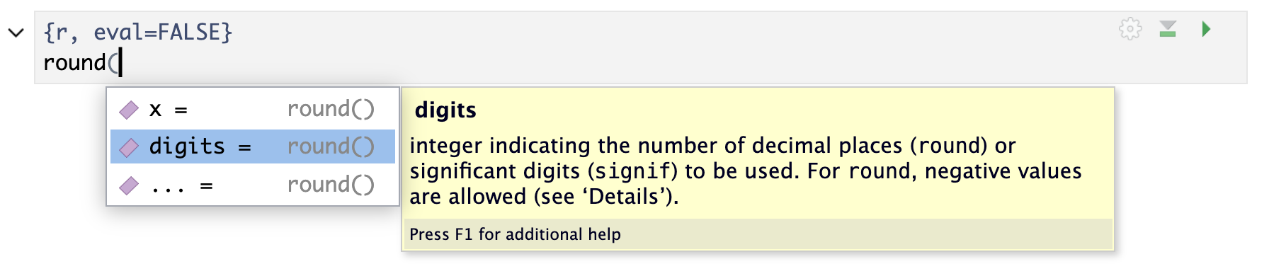
If you try this with the round function, you should see a list of the arguments and if you hover over any one, a description of that parameter

round(<tab>

(Screenshot of tab-complete suggestions)

If you don’t already know the name or beginning of the name of the function you want to use, RStudio’s built in help documentation search function is not always very helpful, and then a Google search is usually better!

2.4.3 Writing functions

In this class, you will be working a lot with functions, especially those that someone else has already written. When you type sum, c(), or mean(), you are using a function that has been made previously and built into R. To remove some of the magic around these functions, we will go through how to make a basic function of our own. Let’s start with a simple example where we add two numbers together:

add_two_numbers <- function(num1, num2) {
    return(num1 + num2)
}
add_two_numbers(4, 5)

[1] 9

As you can see, running this function on two numbers returns their sum. We could also assign to a variable in the function and return the function.

add_two_numbers <- function(num1, num2) {
    my_sum <- num1 + num2
    return(my_sum)
}
add_two_numbers(4, 5)

[1] 9

When you define your own function and run that section of code, the function becomes accessible in your environment, in the same way variables you define do (you should be able to see it in the Environment window in RStudio).

However, variables defined only within a function are not accessible outside that function:

my_sum

Error:
! object 'my_sum' not found

Functions can include calculations of any complexity within them. For example, we can write a function that calculates a person’s BMI from their measured weight (in lbs) and height (in inches) in a multistep process:

get_bmi <- function(weight_lbs,height_inches){
  
  weight_kg <- weight_lbs/2.2 # convert weight from lbs to kg
  height_cm <- height_inches * 2.54 # convert height from inches to cm
  height_m <- height_cm/100 # convert height from cm to m
  bmi <- weight_kg/(height_m^2)  # get BMI
  
  return(bmi)
}

weight_lbs <- 150
height_inches <- 72

get_bmi(weight_lbs, height_inches)

[1] 20.38619

It’s good practice to give the parameters of a function intuitive names and to document the steps with comments as much as possible, so that if you or someone else goes to use your function later, you’ll remember what it does and how.

Check and see that now that you’ve created your own function, it shows up when you use tab-complete with information on the input parameters!

2.4.3.1 Challenge

Can you write a function that calculates the mean of 3 numbers?

2.5 Vectors and data types

2.5.1 Creating vectors

A vector is the most common and basic data type in R, and is pretty much the workhorse of R. A vector is composed by a series of values, which can be either numbers or characters. We can assign a series of values to a vector using the c() function, which stands for “concatenate (combine/connect one after another) values into a vector” For example we can create a vector of animal weights and assign it to a new object weight_g:

weight_g <- c(50, 60, 65, 82) # Concatenate/Combine values into a vector
weight_g

[1] 50 60 65 82

You can also use built-in commands in R to create simple types of numeric vectors, for example:

The semi-colon : creates a vector of numbers increasing by 1 each time

1:10

 [1]  1  2  3  4  5  6  7  8  9 10

The seq function creates a sequence of numbers increasing by a fixed amount

seq(0, 30) # This is the same as just `0:30`

 [1]  0  1  2  3  4  5  6  7  8  9 10 11 12 13 14 15 16 17 18 19 20 21 22 23 24
[26] 25 26 27 28 29 30

seq(0, 30, 3) # Every third number

 [1]  0  3  6  9 12 15 18 21 24 27 30

seq(from = 0, to = 20, by = 2.5) # from 0 to 20 with step size 2.5

[1]  0.0  2.5  5.0  7.5 10.0 12.5 15.0 17.5 20.0

The rep function creates a vector with the same value repeated a specified number of times

rep(0,7)

[1] 0 0 0 0 0 0 0

A vector can also contain characters (i.e., letters) or strings (i.e., words/phrases):

animals <- c('mouse', 'rat', 'dog')
animals

[1] "mouse" "rat"   "dog"

The quotes around “mouse”, “rat”, etc. are essential here and can be either single or double quotes. Without the quotes R will assume there are objects called mouse, rat and dog. As these objects don’t exist in R’s memory, there will be an error message.

There are many functions that allow you to inspect the content of a vector. length() tells you how many elements are in a particular vector:

length(weight_g)

[1] 4

length(animals)

[1] 3

An important feature of a vector is that all of the elements are the same type of data. The function class() indicates the class (the type of element) of an object:

class(weight_g)

[1] "numeric"

class(animals)

[1] "character"

The function str() provides an overview of the structure of an object and its elements. It is a useful function when working with large and complex objects:

str(weight_g)

 num [1:4] 50 60 65 82

str(animals)

 chr [1:3] "mouse" "rat" "dog"

You can use the c() function to add other elements to your vector:

weight_g <- c(weight_g, 90) # add to the end of the vector
weight_g <- c(30, weight_g) # add to the beginning of the vector
weight_g

[1] 30 50 60 65 82 90

In the first line, we take the original vector weight_g, add the value 90 to the end of it, and save the result back into weight_g. Then we add the value 30 to the beginning, again saving the result back into weight_g.

We can do this over and over again to grow a vector, or assemble a dataset. As we program, this may be useful to add results that we are collecting or calculating.

An atomic vector is the simplest R data type and it is a linear vector of a single type, e.g. all numbers. Above, we saw 2 of the 6 main atomic vector types that R uses: "character" and "numeric" (or "double"). These are the basic building blocks that all R objects are built from.

Vectors are one of the many data structures that R uses. Other important ones are lists (list), matrices (matrix), data frames (data.frame), factors (factor) and arrays (array). In this class, we will focus on data frames, which is most commonly used one for data analyses.

2.5.1.1 Challenge

We’ve seen that atomic vectors can be of type character, numeric (or double), integer, and logical. But what happens if we try to mix these types in a single vector? Find out by using class to test these examples.

num_char <- c(1, 2, 3, 'a')
num_logical <- c(1, 2, 3, TRUE)
char_logical <- c('a', 'b', 'c', TRUE)
tricky <- c(1, 2, 3, '4')

This happens because vectors can be of only one data type. Instead of throwing an error and saying that you are trying to mix different types in the same vector, R tries to convert (coerce) the content of this vector to find a “common denominator”. A logical can be turn into 1 or 0, and a number can be turned into a string/character representation. It would be difficult to do it the other way around: would 5 be TRUE or FALSE? What number would ‘t’ be?

In R, we call converting objects from one class into another class coercion. These conversions happen according to a hierarchy, whereby some types get preferentially coerced into other types. Can you draw a diagram that represents the hierarchy of how these data types are coerced?

This can be important to watch for in data sets that you import.

2.5.2 Subsetting vectors

If we want to extract one or several values from a vector, we must provide one or several indices in square brackets. For instance:

animals <- c("mouse", "rat", "dog", "cat")
animals[2]

[1] "rat"

animals[c(3, 2)]

[1] "dog" "rat"

We can also repeat the indices to create an object with more elements than the original one:

more_animals <- animals[c(1, 2, 3, 2, 1, 4)]
more_animals

[1] "mouse" "rat"   "dog"   "rat"   "mouse" "cat"

R indices start at 1. Programming languages like Fortran, MATLAB, Julia, and R start counting at 1, because that’s what human beings typically do. Languages in the C family (including C++, Java, Perl, and Python) count from 0 because that was historically simpler for computers and can allow for more elegant code in some situations.

2.5.3 Conditional subsetting

Another common way of subsetting is by using a logical vector. TRUE will select the element with the same index, while FALSE will not:

weight_g <- c(21, 34, 39, 54, 55)
weight_g[c(TRUE, FALSE, TRUE, TRUE, FALSE)]

[1] 21 39 54

Typically, these logical vectors are not typed by hand, but are the output of other functions or logical tests. For instance, if you wanted to select only the values above 50:

weight_g > 50    # will return logicals with TRUE for the indices that meet the condition

[1] FALSE FALSE FALSE  TRUE  TRUE

## so we can use this to select only the values above 50
weight_g[weight_g > 50]

[1] 54 55

We will consider conditions in more detail in the next few lectures.

2.5.4 Strings and character vectors

Just a small note about character vectors, also called strings. There are built-in packages for subsetting them that we’ll learn about later. They can be particularly relevant for ecological/genomics because important data can be nested in complicated strings of text (ex: extracting only the observations that occurred in wet habitats from a column of habitat descriptions or only genes with functions related to drought tolerance).

string1 <- "This is a string" # you can include spaces between your quotes
string2 <- c(string1, "so is this") # concatenate with another string
string2[2] # can access the second string via subsetting

[1] "so is this"

# Playing a bit with declaring variables
"You can include 'quotes' in a string"

[1] "You can include 'quotes' in a string"

string3 <- 'You can include "quotes" in a string'
string3

[1] "You can include \"quotes\" in a string"

"You can include \"matching quotes\" if you 'escape' them with a backslash (\\)"

[1] "You can include \"matching quotes\" if you 'escape' them with a backslash (\\)"

You can combine two separate strings into a single string using the paste function

paste("Julius","Caesar")

[1] "Julius Caesar"

paste("pan","cake",sep="")

[1] "pancake"

Which can also be used to convert a vector of strings back into a single string

emperor <- c("Julius","Caesar")
paste(emperor, collapse = " ")

[1] "Julius Caesar"

2.6 Loops and if/else statements

Loops, specifically for-loops, are essential to programming. They allow us to follow a formula to do a repeated task in a systematic way. You can think of a for-loop as: “for each number contained in a list/vector, perform this operation” and the syntax basically says the same thing:

v <- c(2, 4, 6)
for (num in v) {
    print(num)
}

[1] 2
[1] 4
[1] 6

Instead of printing out every number to the console, we could also add numbers cumulatively, to calculate the sum of all the numbers in the vector:

# To increment `w` each time, we must first create the variable,
# which we do by setting `w <- 0`, referred to as initializing.
# This also ensures that `w` is zero at the start of the loop and
# doesn't retain the value from last time we ran this code.
w <- 0
for (num in v) {
    w <- w + num
}
w

[1] 12

If we put what we just did inside a function, we have essentially recreated the sum function in R.

my_sum <- function(input_vector) {
    vector_sum <- 0
    for (num in input_vector){
        vector_sum <- vector_sum + num
    }
    return(vector_sum)
}

my_sum(v)

[1] 12

Although this gives us the same output as the built-in function sum, the built-in function has many more optimizations so it is much faster than our function.

In general, in R, it is always faster to try to find a way of doing things without writing a loop yourself, if possible. When you are reading about R, you might see suggestions that you should try to vectorize your code to make it faster. What people are referring to, is that you should not write for loops in R and instead use the ready-made functions that are much more efficient in working with vectors and essentially performs operations on entire vector at once instead of one number at a time. Conceptually, loops operate on one element at a time while vectorized code operates on all elements of a vector at once. However, sometimes there is no vectorized way of going about what you want to do (or at least, no easy, obvious, or quick-to-code vectorized way!).

For some calculations we can’t easily avoid for-loops. For example, let’s generate the first 25 values of the Fibonacci sequence

fib_vec <- rep(0,25)
fib_vec[c(1,2)] <- c(0,1)

for (i in 3:25){
  fib_vec[i] <- fib_vec[i-2]+fib_vec[i-1]
}

fib_vec

 [1]     0     1     1     2     3     5     8    13    21    34    55    89
[13]   144   233   377   610   987  1597  2584  4181  6765 10946 17711 28657
[25] 46368

R also provides two other types of loops that can be helpful for repetitive or recursive tasks: while-loops (which continue iterating while a statement is true) and repeat loops (which continue repeating until a certain break condition is met).

Another very useful programming structure we can use in R, which is often combined with for-loops, is if/else statements. We can use this approach to only do an operation on an object if a certain condition is met, and do an alternative operation if the condition is not met.

For example, we could loop through a vector of ages and classify each individual as either an adult or a child

ages <- c(67,13,45,3,7,34,90,8)
age_cat <-rep("",length(ages)) # set up an empty character vector

for (i in 1:length(ages)){
  
  if (ages[i] < 18){
    age_cat[i] <- "child"
  }else{
    age_cat[i] <- "adult"
  }
  
}

print(age_cat)

[1] "adult" "child" "adult" "child" "child" "adult" "adult" "child"

For simple if/else statements, R provides a shorter notation

ages <- c(67,13,45,3,7,34,90,8)
age_cat <-rep("",length(ages)) # set up an empty character vector

for (i in 1:length(ages)){
  
  age_cat[i] <- ifelse(ages[i] < 18,"child","adult")
  
}

print(age_cat)

[1] "adult" "child" "adult" "child" "child" "adult" "adult" "child"

For more complex criteria, multiple “else” statements can be used:

ages <- c(67,13,45,3,7,34,90,8)
age_cat <-rep("",length(ages)) # set up an empty character vector

for (i in 1:length(ages)){
  
  if (ages[i] < 18){
    age_cat[i] <- "child"
  }else if (ages[i] < 65){
    age_cat[i] <- "adult"
  }else{
    age_cat[i] <- "senior"
  }
  
}

print(age_cat)

[1] "senior" "child"  "adult"  "child"  "child"  "adult"  "senior" "child"

Note that this is an example of a computation that could be sped up by vectorization:

ages <- c(67,13,45,3,7,34,90,8)
age_cat <-rep("",length(ages))

age_cat[ages<18] <-"child"
age_cat[ages>18 & ages<65] <-"adult"
age_cat[ages>65] <-"senior"
age_cat

[1] "senior" "child"  "adult"  "child"  "child"  "adult"  "senior" "child"

# OR
# age_cat <- ifelse(ages < 18, "child",ifelse(ages>65, "senior", "adult"))

Refer to the tidy style guide for which style to adhere to.↩︎
There are a few other symbols as well, all of which can be viewed at the end of this post about RStudio code completion.↩︎