install.packages("tinytex")
tinytex::install_tinytex()1 Downloading and installing R
1.1 Introduction
This course uses R, a computing environment that combines numerical analysis tools for linear algebra, a wide range of scientific computing algorithms, functions for classical and modern statistical analysis; and functions for graphics and data visualization. It is based on the programming language S, developed by John Chambers in the 1970s. Today, R is most popular among statisticians, data scientists, biologists, and public health researchers, but is used broadly across many fields.
We will use the graphical user interface (GUI) to R, a software called RStudio, throughout this course. Although the GUI makes many tasks easier, it is not necessary to use it when running R. Both methods will be described below.
1.2 Installing R
Download R, a free software environment for statistical computing and graphics from CRAN, the Comprehensive R Archive Network. Use the links specific to your operating system at the top of the page (i.e., the `precompiled binary distribution’).
For Mac users: Select the
.pkgfile for the latest R version. Mac users with an Apple Silicon chip (e.g., M1 or M2) should install the “arm64” version of R, while Mac users with an Intel chip should install the regular (64-bit) version of R. You can check your laptop’s hardware specifications by clicking the Apple icon (top left corner)\> About This Mac. Once the.pkgfile is downloaded to your computer, double click it and follow the prompts to install RFor Windows users: Select the
basefile and download. Run the.exefile that was just downloaded and follow the instructions on screen to install the downloaded software locally on your computer.For Linux users: Follow the links and instructions provided for your distribution
If you previously downloaded R for another class or purpose, check what version you have. For maximum compatibility with the code provided for the class, ensure that the R version is 4.5.2 (the latest). You can check your R version by opening the R program (or RStudio if you already have it), and at the prompt (indicated by the > ) typing version. If you have an out-of-date version, you have to download a new one following the instructions above (there’s no separate update process).
{width=50%}
No laptop? No problem! If you don’t have a laptop computer that allows you to install software (e.g., a tablet or Chromebook), or if your laptop is older and difficult to run resource-heavy programs, you can instead access R and RStudio from your web browser and do you your computations in the cloud using the cloud-based version of RStudio, called POSIT Cloud. Sign up for a free account here. We’ll add you to our EEB313 workspace so you’ll get more cloud credits than a regular free account.
1.3 Installing RStudio
Download and install RStudio by choosing your specific operating system, then following the instructions to download the software package and install it for your operating system.
Note: If your have previously installed RStudio but newer versions have been released, it will automatically notify you and provide the link to update it. There is no connection between versions of R and RStudio - you have to update them independently. If you are updating your version of R after opening R Studio, make sure R Studio is restarted and then verify it recognizes the most recent version of R. On Macs, this is usually automatic, but on Windows, it is possible to have multiple versions of R installed, so if you didn’t delete an older version in the process of installing the new one, you might have to tell RStudio which version of R to use.
1.5 Coding in R
Within RStudio, there are a few ways we can run code in R.
For short commands that we aren’t likely to want to repeat, we can simply type then into the console, and the answer will be returned immediately, e.g.
> 1+2
We can similarly to a series of calculations where the current one depends on the prior. However, this method becomes inconvenient for all but the simplest calculations, since it’s more difficult to repeat a series of calculations in an automated way. For this reason, it is more common to write commands in scripts. Scripts are simply series of lines of code saved in a text file.
To create a new script, go to File > New File > RScript, give it a name (like my_test.R), and save it. Once you have written the code you want, there are a few ways you can actually get it to run
using your cursor to highlight all the code text, and then hitting the icon with the green forward arrow and the word `Run’ in the top right of the scripts panel
typing
>source('mytest.R')at the prompt in the RStudio console
Both methods result in the same code being run, although in the latter method, the result of each calculation will not be printed off to the console. You need to enclose the statement you wanted displayed in the print() command, i.e. print(2+3)
Comments! Running any code with a # at the beginning of the line results in the line being read as a comment. This means that the calculation which is specified in the line is not processed and the output not returned. Comments are a useful way to keep track of what line(s) of code do, multiple versions of the same code, etc. Usually we use them to make notes about what the code following the comment is doing and why. Its the most basic way of documenting code for others who may use it (as well as our future selves). However, comments are very limited, since they can’t include any text formatting, so for most of this course we’ll instead be using a different type of R script document called a notebook, which allows us to use the R Markdown format, for much nicer documentation and presentation of our results.
Installing R packages
R packages are basically bundles of functions that perform related tasks. There are many some that will be come with a base install of R since they are considered critical for using R, such as c(), mean(), +, -, etc.
There is an official repository for R-packages beyond the base packages called CRAN (Comprehensive R Archive Network). CRAN has thousands of packages, and all these cannot be installed by default, because then base R installation would be huge and most people would only be using a fraction of everything installed on their machine. It would be like if you downloaded the Firefox or Chrome browser and you would get all extensions and add-ons installed by default, or as if your phone came with every app ever made for it already installed when you bought it: quite impractical.
Instead, individual users tend to download and install only the packages they really need for their work. While this may be efficient in terms of the space in memory taken up by the app, it can lead to some challenges when sharing code, if you’re not careful to ensure that the code is documented to specify the required packages, and to autmoatically download and install then if they’re missing.
1.5.1 TinyTex
There is one package we have to install first before we can create PDF reports, which will be necessary for assignments and the project (the default is to create HTML reports, which can be opened in any web browser, and are useful to make some sorts of interactive visuals, but are not as easy to share and view as PDFs). Copy and paste into the console (where the \> symbol is) the two lines of code below to install a package called tinytex.
1.5.2 Tidyverse
tidyverse1 is a large collection of packages with similar functions, similar to the way Microsoft Word is part of Microsoft Office. tidyverse, as its name may suggest, contains many packages that makes data cleaning and exploring more intuitive and effective. It is basically an entire philosophy on how to handle data and has a massive following.
The two tidyverse packages we will be using the most frequently in this course is dplyr and ggplot2. dplyr is great for data wrangling (Lecture 3) and ggplot2 makes killer plots (Lecture 4).
- Copy and paste the below code into your console.
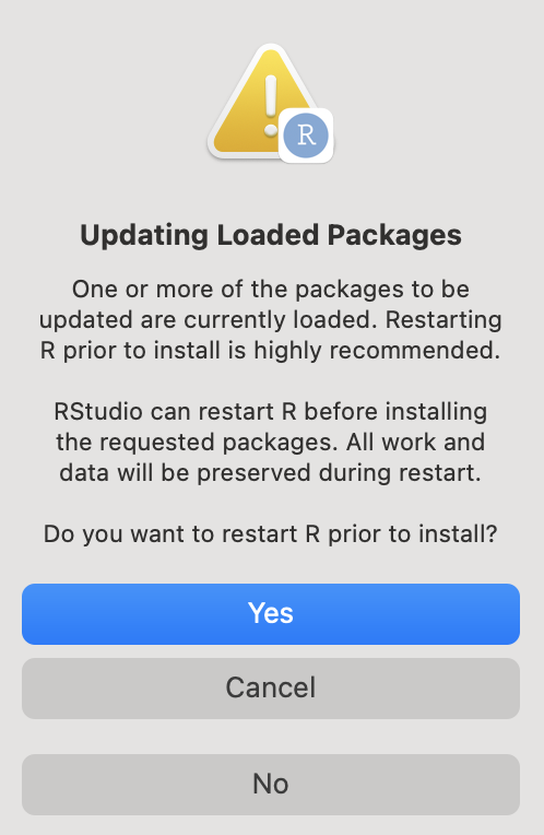
install.packages(c("tidyverse", "data.table"), dependencies = TRUE)During installation, if you ever get the below message, click “No”.
If you get the message “Do you want to install from sources the packages which need compilation? (Yes/no/cancel)” in the Console, type “Yes” and press enter.
- Check that the tidyverse package has been installed correctly. To do this, go to the bottom right pane and click the tab for “Packages”. If you can search for and find the below packages, then they have been installed! They do not need to be checked off. Alternatively, go to the Console and type
library(tidyverse)to verify that the package is installed. An error along the lines “there is no package called tidyverse” will be returned if the package is not installed.
1.6 R Notebooks and R Markdown
1.6.1 Creating R notebooks
In the RStudio interface, we will be writing code in a format called the R Notebook. As the name entails, this interface works like a notebook for code, as it allows us to save notes about what the code is doing, the code itself, and any output we get, such as plots and tables, all together in the same document.
In RStudio you can create a new R Markdown notebook by going to File > R Markdown. It will appear in the same panel as scripts. The file name should end in .Rmd. - Read the guidelines provided in example text in that notebook.
When we are in the notebook, the text we write is normal plain text, just as if we would be writing it in a text document. If we want to execute some R code, we need to insert a code chunk.
You insert a code chunk by either clicking the “Insert” button (icon with a green +C in the top right) or pressing Command + Option + i (on Mac/Linux, or Ctrl + Alt + i on Windows) simultaneously. You could also type out the surrounding backticks, but this would take longer. To run a code chunk, you press the green arrow, or Ctrl/Command + Shift + Enter.
1+2[1] 3As you can see, the output appears right under the code block.
This is a great way to perform explore your data, since you can do your analysis and write comments and conclusions right under it all in the same document. A powerful feature of this workflow is that there is no extra time needed for code documentation and note-taking, since you’re doing your analyses and taking notes at the same time. This makes it great for both taking notes at lectures and to have as a reference when you return to your code in the future.
1.6.2 R Markdown
The text format we are using in the R Notebook is called R Markdown. This format allows us to combine R code with the Markdown text format, which enables the use of certain characters to specify headings, bullet points, quotations and even citations. A simple example of how to write in Markdown is to use a single asterisk or underscore to emphasize text (*emphasis*) and two asterisks or underscores to strongly emphasize text (**strong emphasis**). When we convert our R Markdown text to other file formats, these will show up as italics and bold typeface, respectively. If you have used WhatsApp, you might already be familiar with this style of writing. In case you haven’t seen it before, you have just learned something about WhatsApp in your quantitative methods class…
To learn more about R Markdown, check out this reference. More helpful commands are also provided in the [EEB R Manual](https://rman.eeb.utoronto.ca/basic-r/rmarkdown/)
1.6.3 Saving data and generating reports
To save our notes, code, and graphs, all we have to do is to save the R Markdown file, and the we can open it in RStudio next time again. However, if we want someone else to look at this, we can’t always just send them the R Notebook file, because they might not have RStudio installed. Another great feature of R Notebooks is that it is really easy to export them to HTML, Microsoft Word, or PDF documents with figures and professional typesetting. There are actually many academic papers that are written entirely in this format and it is great for assignments and reports. (You might even use it to communicate with your collaborators!) Since R Notebook files convert to HTML, it is also easy to publish simple and good-looking websites in it, in which code chunks are embedded nicely within the text.
Let’s try to create a document in R.
First, let’s set up the YAML block. This is found at the top of your document, and it is where you specify the title of your document, what kind of output you want, etc.
---
title: "Your title here"
author: "Your name here"
date: "Insert date"
output:
  pdf_document: default
---
If you are interested in playing with other YAML options, check out this guide.
Next, let’s type code to perform the calculation we did above:
1+2[1] 3To create the output document, we say that we “knit” our R Markdown file into, e.g., a PDF. Simply press the Knit button here and the new document will be created. The first time you do this, you might be asked to install some R packages if it’s the first time you’ve done this - go ahead an let them install.
As you can see in the knitted document, the title showed up as we would expect, and lines with pound sign(s) in front of them were converted into headers. Most importantly, we can see both the code and its output! Plots are generated directly in the report without us having to cut and paste images! If we change something in the code, we don’t have to find the new images and paste it in again, the correct one will appear right in your code.
When you quit, R will ask you if you want to save the workspace (that is, all of the variables you have defined in this session); in general, you should say “no” to avoid clutter and unintentional confusion of results from different sessions. Note: When you say “yes” to saving your workspace, it is saved in a hidden file named .RData. By default, when you open a new R session in the same directory, this workspace is loaded and a message informing you so is printed: [Previously saved workspace restored]. It is often best practice to turn this feature off completely.
1.6.4 A quick note on variables and memory in R notebooks
When you run code in a notebook by simply interacting with the text in the notebook text file (ie via clicking the green `run’ arrow or typing Command+Shift+Enter, any variables or other objects you create will be available in your RStudio projects environment (i.e. viewable in the Environment pane and accessible via the console). However, when you run a document by knitting, it is actually running a separate, private, session of R, and so the output cannot be accessed later. If you want to examine any output produced in a notebook that’s knitted, make sure the notebook itself contains commands to print the objects so they can be seen in the kitted form.
This course is focused on
tidyversefunctions, because that seems to be the trend these days. Although all of our teaching material is written in tidy lingo, it is mostly for the sake of consistency. In all honesty, tidy is pretty great, but some functions are more intuitive in base, so most people code in a mix of the two. If you learned base R elsewhere and prefer to use those functions instead, by all means, go ahead. The correct code is code that does what you want it to do.↩︎